Plot of HazardShape objects

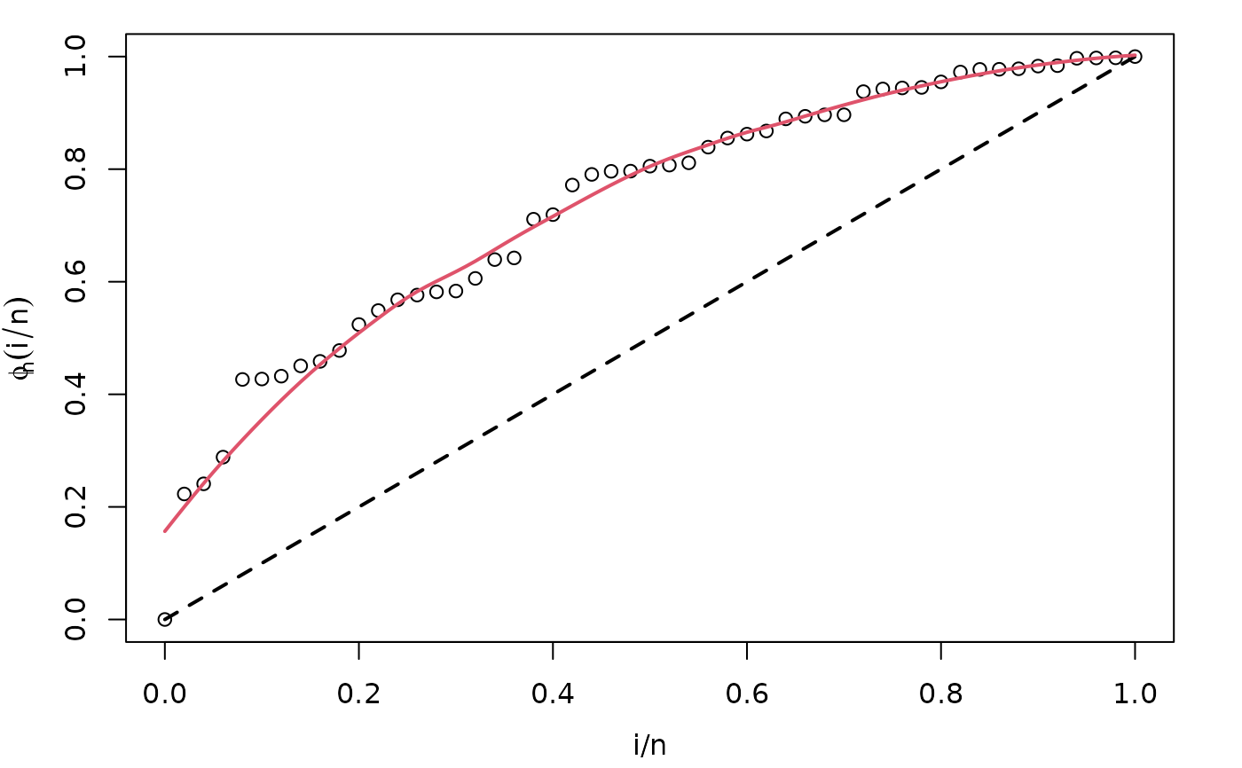
Draws the empirical total time on test (TTT) plot and its non-parametric (LOESS) estimated curve useful for identifying hazard shape.

Usage

# S3 method for HazardShape
plot(
  x,
  xlab = "i/n",
  ylab = expression(phi[n](i/n)),
  xlim = c(0, 1),
  ylim = c(0, 1),
  col = 1,
  lty = NULL,
  lwd = NA,
  main = "",
  curve_options = list(col = 2, lwd = 2, lty = 1),
  par_plot = lifecycle::deprecated(),
  legend_options = lifecycle::deprecated(),
  ...
)

Arguments

x

an object of class initValOW, generated with TTT_hazard_shape.

xlab, ylab

titles for x and y axes, as in plot.

xlim

the x limits (x1, x2) of the plot.

ylim

the y limits (x1, x2) of the plot.

col

the colors for lines and points. Multiple colors can be specified. This is the usual color argument of plot.default.

lty

a vector of line types, see par for further information.

lwd

a vector of line widths, see par for further information.

main

a main title for the plot.

curve_options

a list with further arguments useful for customization of non-parametric estimate plot.

par_plot

(deprecated) some graphical parameters which can be passed to the plot. See Details section for further information.

legend_options

(deprecated) a list with fur further arguments useful for customization. See Details section for further information. of the legend of the plot.

...

further arguments passed to empirical TTT plot.

Details

This plot complements the use of TTT_hazard_shape. It is always advisable to use this function in order to check the result of non-parametric estimate of TTT plot. See the first example in Examples section for an illustration.

Author

Jaime Mosquera Gutiérrez jmosquerag@unal.edu.co

Examples

library(EstimationTools)

#----------------------------------------------------------------------------
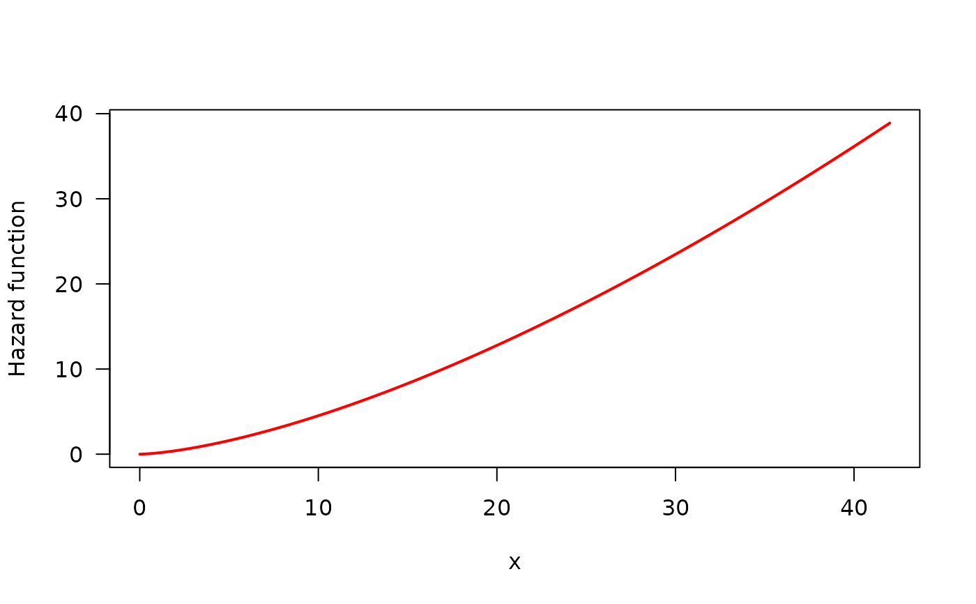
# Example 1: Increasing hazard and its corresponding TTT plot with simulated
# data
hweibull <- function(x, shape, scale) {
  dweibull(x, shape, scale) / pweibull(x, shape, scale, lower.tail = FALSE)
}
curve(hweibull(x, shape = 2.5, scale = pi),
  from = 0, to = 42,
  col = "red", ylab = "Hazard function", las = 1, lwd = 2
)


y <- rweibull(n = 50, shape = 2.5, scale = pi)
my_initial_guess <- TTT_hazard_shape(formula = y ~ 1)

par(mar = c(3.7, 3.7, 1, 2), mgp = c(2.5, 1, 0))
plot(my_initial_guess)


#----------------------------------------------------------------------------