Plot method for EmpiricalTTT objects

Draws a TTT plot of an EmpiricalTTT object, one for each strata.

TTT plots are graphed in the same order in which they appear in the list element strata or in the list element phi_n of the EmpiricalTTT object.

Usage

# S3 method for EmpiricalTTT
plot(
  x,
  add = FALSE,
  grid = FALSE,
  type = "l",
  pch = 1,
  xlab = "i/n",
  ylab = expression(phi[n](i/n)),
  ...
)

Arguments

x

an object of class EmpiricalTTT.

add

logical. If TRUE, plot.EmpiricalTTT add a TTT plot to an already existing plot.

grid

logical. If TRUE, plot appears with grid.

type

character string (length 1 vector) or vector of 1-character strings indicating the type of plot for each TTT graph. See plot.

pch

numeric (integer). A vector of plotting characters or symbols when type = "p". See points.

xlab, ylab

titles for x and y axes, as in plot.

...

further arguments passed to matplot. See the examples and Details section for further information.

Details

This method is based on matplot. Our function sets some default values for graphic parameters: type = "l", pch = 1, xlab = "i/n" and ylab = expression(phi[n](i/n)). This arguments can be modified by the user.

See also

TTTE_Analytical, matplot

Author

Jaime Mosquera Gutiérrez, jmosquerag@unal.edu.co

Examples

library(EstimationTools)

#--------------------------------------------------------------------------------
# First example: Scaled empirical TTT from 'mgus1' data from 'survival' package.

TTT_1 <- TTTE_Analytical(Surv(stop, event == 'pcm') ~1, method = 'cens',
                         data = mgus1, subset=(start == 0))
plot(TTT_1, type = "p")



#--------------------------------------------------------------------------------
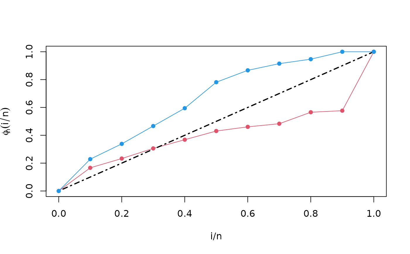
# Second example: Scaled empirical TTT using a factor variable with 'aml' data
# from 'survival' package.

TTT_2 <- TTTE_Analytical(Surv(time, status) ~ x, method = "cens", data = aml)
plot(TTT_2, type = "l", lty = c(1,1), col = c(2,4))
plot(TTT_2, add = TRUE, type = "p", lty = c(1,1), col = c(2,4), pch = 16)


#--------------------------------------------------------------------------------
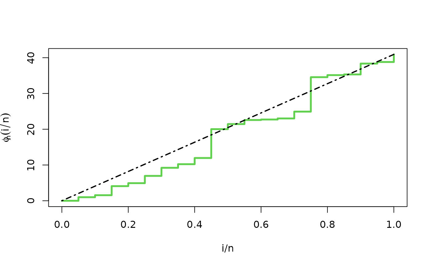
# Third example: Non-scaled empirical TTT without a factor (arbitrarily simulated
# data).

y <- rweibull(n=20, shape=1, scale=pi)
TTT_3 <- TTTE_Analytical(y ~ 1, scaled = FALSE)
plot(TTT_3, type = "s", col = 3, lwd = 3)



#--------------------------------------------------------------------------------
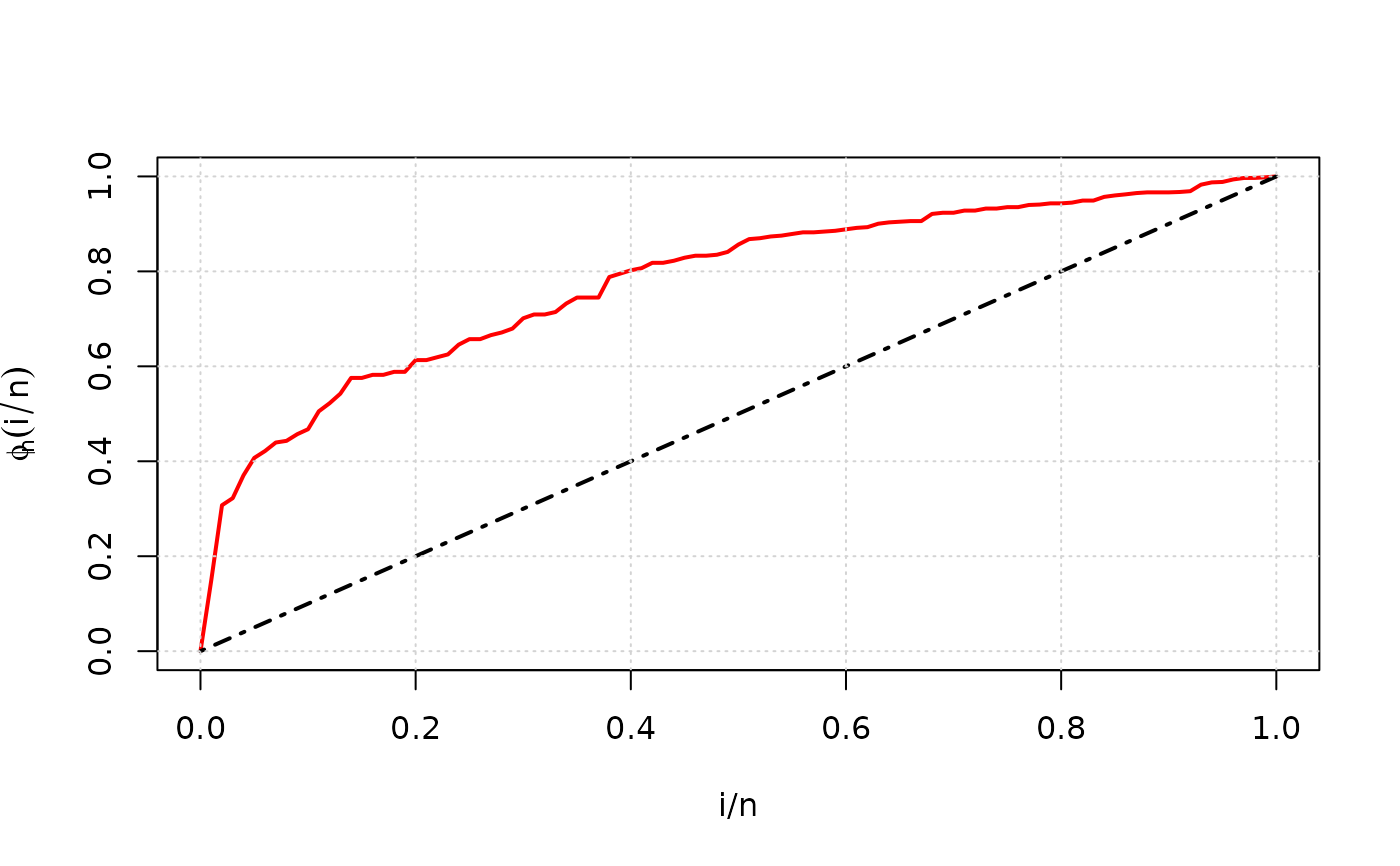
# Fourth example: TTT plot for 'carbone' data from 'AdequacyModel' package

if (!require('AdequacyModel')) install.packages('AdequacyModel')
#> Loading required package: AdequacyModel
library(AdequacyModel)
data(carbone)
TTT_4 <- TTTE_Analytical(response = carbone, scaled = TRUE)
plot(TTT_4, type = "l", col = "red", lwd = 2, grid = TRUE)



#--------------------------------------------------------------------------------